


[Contribution] Understanding the Difficult Millimeter-Wave System Design (Part 1)
 Published2017.08.18 15:13
Cesar Iovescu / 레이더 애플리케이션 관리자
밀리미터파(mmWave)는 단파장의 전자파를 사용하는 특수한 등급의 레이더 기술이다. 레이더 시스템은 경로에 있는 물체에 전자파 신호를 보낸 후 반사시킨다. 반사 신호를 포착하면 물체의 범위, 속도, 각도를 파악할 수 있다.
mmWave 레이더는 밀리미터 범위 내에 있는 파장을 사용하여 신호를 보낸다. 이는 전자기 스펙트럼에서 단파장으로 간주되며, 이 기술의 이점 중 하나다. 실제로 mmWave 신호를 처리하는 데 필요한 안테나와 같은 시스템 구성 요소의 크기는 작다. 단파장의 또 다른 이점은 높은 정확도다. 76~81GHz에서 작동하는 mmWave 시스템(해당 파장은 약 4mm) 은 1밀리미터의 몇 분의 1에 불과한 작은 움직임도 감지할 수 있다.
완전한 mmWave 레이더 시스템에는 전송(TX) 및 수신(RX) 라디오 주파수(RF) 구성요소, 클로킹과 같은 아날로그 구성 요소, ADC(아날로그-디지털 컨버터), MCU(마이크로컨트롤러) 및 DSP(디지털 신호 프로세서)와 같은 디지털 구성 요소가 포함된다. 기존에는 이러한 시스템이 개별 구성 요소로 구현되어 소비 전력과 전반적인 시스템 비용이 증가했다. 복잡성과 고주파 때문에 시스템 설계도 까다로웠다.
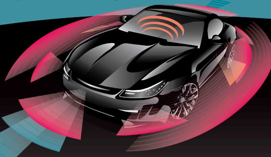
텍사스 인스트루먼트(TI)는 이러한 과제를 해결하고, 클로킹과 같은 TX-RF 및 RX-RF 아날로그 구성 요소와 ADC, MCU 및 하드웨어 액셀러레이터와 같은 디지털 구성요소를 통합하는 CMOS(상보성 금속 산화막 반도체) 기반의 mmWave 레이더 디바이스를 설계했다. TI mmWave 센서 포트폴리오의 일부 제품군은 추가 신호 처리 기능을 위해 DSP를 통합했다.
TI 디바이스는 FMCW(주파수 변조된 연속파)라고 하는 특수한 등급의 mmWave 기술을 구현한다. FMCW 레이더는 이름이 의미하듯 주파수 변조된 신호를 연속적으로 전송하여 범위와 각도, 속도를 측정한다. 짧은 펄스를 주기적으로 전송하던 기존의 펄스 레이더 시스템과는 다르다.
범위 측정
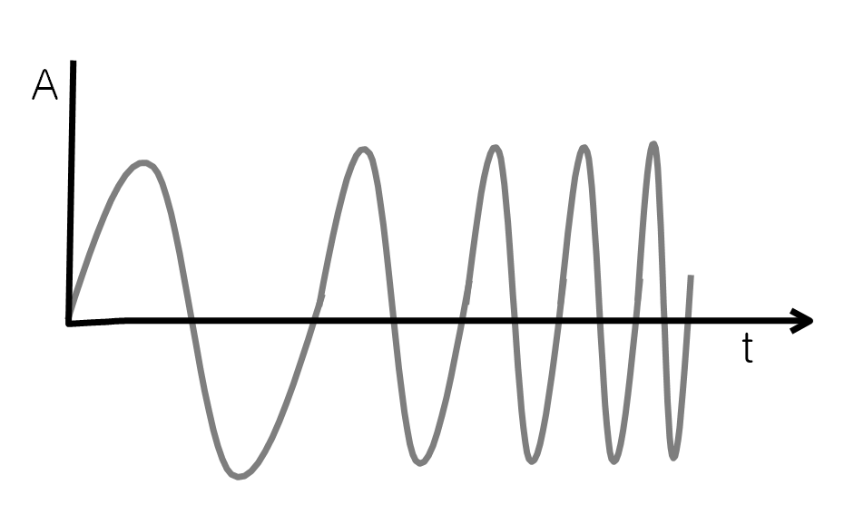
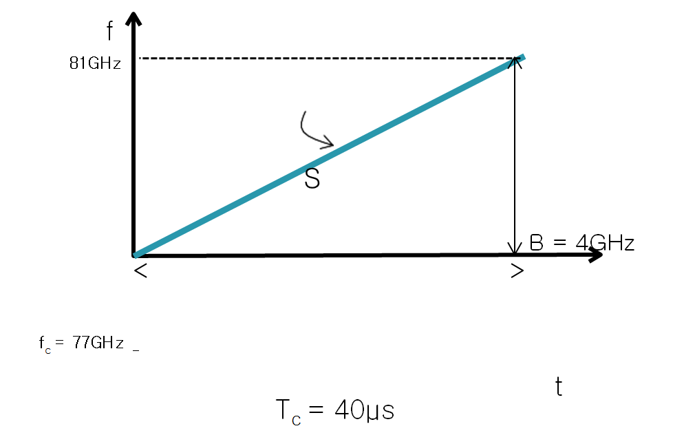
그림 2에는 주파수를 시간 함수로 사용하는 동일한 처프 함수가 나와 있다. 이 처프는 시작 주파수(fc), 대역폭(B) 및 기간(Tc)으로 특성이 결정된다. 처프 기울기 캡처 주파수 변경 속도.
예를 들어 그림 2에 나와 있는 예에서 fc=77GHz, B=4GHz, Tc=40μs, S=100MHz/μs다.
FMCW 레이더 시스템은 처프 신호를 전송한 후 경로에 있는 물체가 반사한 신호를 포착한다. 그림 3에는 FMCW 레이더의 주 RF 구성 요소를 단순하게 표현한 블록 다이어그램이 나와 있다. 레이더는 다음과 같이 작동한다.
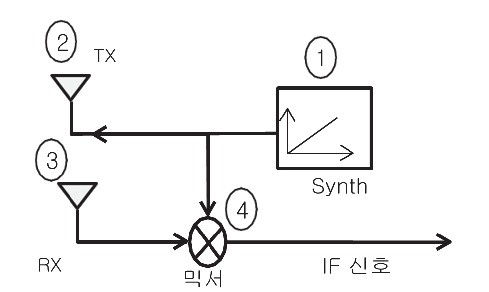
-신시사이저(synth)가 처프를 생성한다.
주파수 믹서는 두 신호를 결합하여 새로운 주파수를 가진 새로운 신호를 만드는 전자 부품이다.
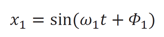
(1)
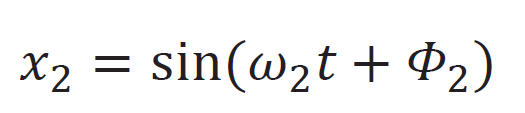
xout 출력은 두 입력 시누소이드의 순시 주파수 차와 동일한 순시 주파수를 가진다. xout 출력의 위상은 두 입력 신호 위상의 차와 같다(방정식 3).

그래픽에서 시간 함수로 표현된 TX 및 RX 처프 주파수를 통해 주파수 믹서의 작동을 이해할 수도 있다.
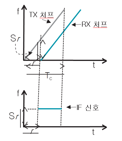
그림 4에서 위쪽 다이어그램은 감지된 단일 물체에 대한 시간 함수로 표현된 TX 및 RX 처프를 보여준다. RX 처프는 TX 처프의 시간 지연 버전이다.
시간 지연(τ)은 방정식 4와 같이 수학적으로 계산할 수 있다.
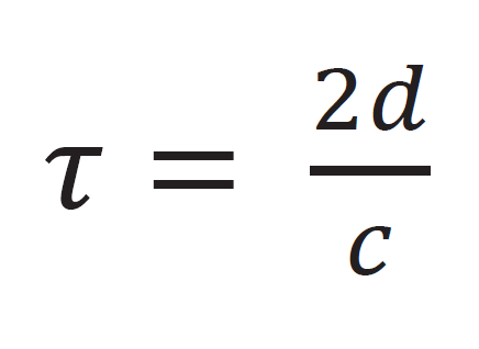 (4)
(4)여기서 d는 감지된 물체와의 거리이고, c는 빛의 속도다.
시간 함수로 표현된 주파수를 구하려면 주파수 믹서 출력 시 IF 신호의 그림 4의 위쪽 섹션에 표시된 두 선을 뺀다. 두 선 사이의 거리는 고정되어 있으므로 IF 신호는 정주파를 가진 톤으로 구성된다. 그림 4는 이 주파수가 Sτ임을 보여준다. IF 신호는 TX 처프와 RX 처프가 겹치는 시간 간격에서만 유효하다(즉, 그림 4의 세로 점선 사이의 간격).

시간 규모 함수로 표현된 믹서 출력 신호는 정주파를 가지므로 사인파다.
IF 신호의 초기 위상(Φ0)은 IF 신호의 시작에 해당하는 순시치에 TX 처프 위상과 RX 처프 위상 사이의 차이다(즉, 그림 4에서 왼쪽 세로 점선으로 표현된 순시치). (방정식 5):
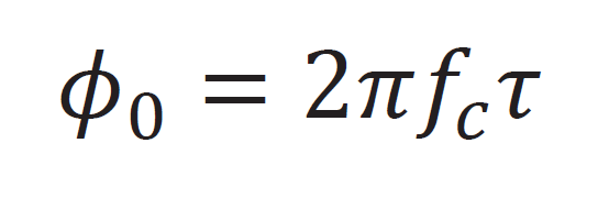 (5)
(5)방정식 6과 같이 수학적으로 계산할 수도 있다.
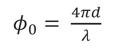 (6)
(6)요약하자면, 레이더와 d거리에 있는 물체의 경우 IF 신호는 사인파다(방정식 7).
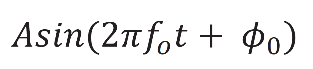 (7)
(7)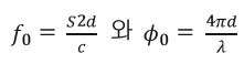 에서,
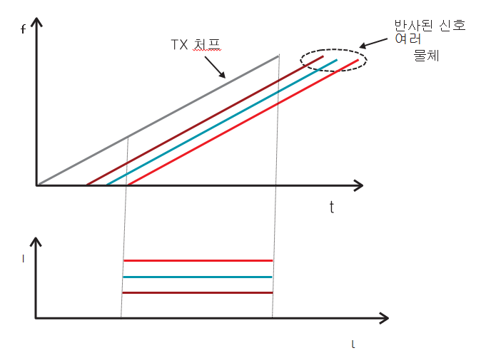
에서,지금까지는 레이더가 한 물체만 감지했다고 가정했다. 이제 여러 개의 물체가 감지된 경우를 분석해 보자. 그림 5에서는 여러 물체에서 수신된 세 가지 RX 처프를 보여준다. 각 처프는 해당 물체와의 거리에 비례한 시간만큼 지연된다. 다양한 RX 처프는 각각 정주파를 가진 여러 IF 톤으로 변환된다.
여러 톤으로 구성된 이 IF 신호는 여러 톤을 구분하기 위해 푸리에 변환을 사용하여 처리되어야 한다. 푸리에 변환 처리 후 여러 톤에 대한 개별 피크가 있는 주파수 스펙트럼이 생성되고, 각 피크는 특정 거리에 있는 물체의 존재를 나타낸다.
범위 분해능
IF 신호의 길이를 늘리려면 대역폭도 그에 비례하여 늘려야 한다. IF 신호의 길이가 늘어나면 별도의 피크가 두 개 있는 IF 스펙트럼이 생성된다.
또한 푸리에 변환 이론에 따르면 관찰 기간(T)을 통해 1/THz 이상의 간격으로 구분된 주파수 구성 요소를 확인할 수 있다. 즉, 주파수가 제시된 관계를 만족할 경우 주파수로 두 IF 신호 톤을 확인할 수 있다. 방정식 8:
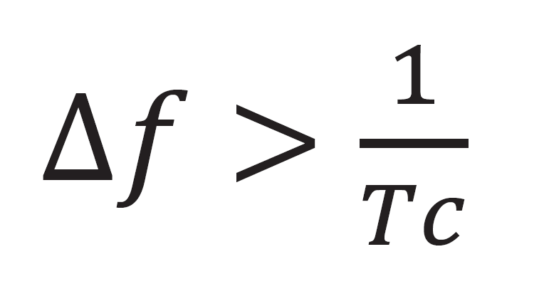 (8)
(8)여기서 Tc는 관찰 간격이다. 따라서,
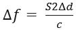
방정식 8은 다음과 같이 표현할 수 있다.
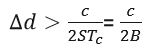
(B=STc이기 때문)
범위 분해능(dRes)은 처프가 휩쓸고 간 대역폭에만 종속된다(방정식 9).
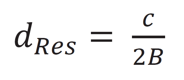 (9)
(9)따라서 처프 대역폭이 몇 GHz인 FMCW 레이더는 센티미터 단위의 범위 분해능을 갖게 된다(예: 4GHz의 처프 대역폭은 3.75cm의 범위 분해능으로 변환된다).
속도 측정
두 처프를 사용한 속도 측정
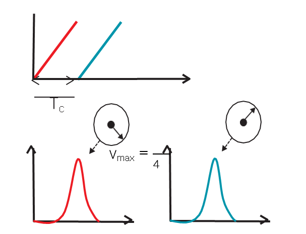
위상 차이는 방정식 10과 같이 방정식 6으로 구한다.
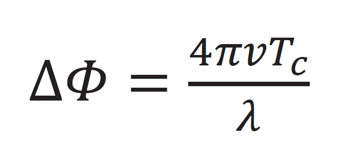 (10)
(10)방정식 11을 사용하여 속도를 구할 수 있다.
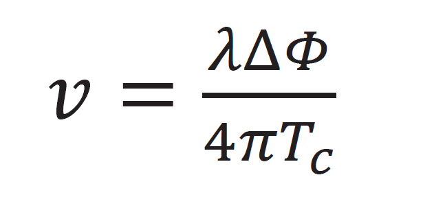 (11)
(11)이 속도 측정은 위상 차이를 기준으로 하므로 모호하다. 이 측정은 |ΔΦ|<π일 경우에만 모호하지 않다. 위의 방정식 11을 사용하여 다음을 수학적으로 계산할 수 있다.
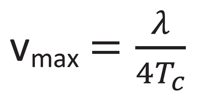 (12)
(12)[다음주중에 까다로운 밀리미터파 시스템 설계 이해하기(하) 나머지 글이 이어집니다]

Comments
Related news
[Feature - Autonomous Vehicles ②] Radar IC Market Seeing More 'Players'; Will Competition Heat Up Among Semiconductor Companies?
If there is a technology where the phrase "dreams have become reality" fits best, it would surely be autonomous vehicles. You summon a car and it comes running on its own, then drives to your destination by itself. Autonomous vehicles recognize and avoid obstacles during driving while providing various convenities and information to the owner. While full autonomy commercialization will take some time, so-called "semi-autonomous driving" technology is becoming increasingly sophisticated. Nowadays, advertisements for automobiles equipped with autonomous driving functions are easy to see, bringing the technology deep into our daily lives. This publication will serialize an autonomous vehicle planning series over the course of 11 installments. Beginning with autonomous vehicle industry trends, we will cover semiconductor components such as radar, lidar, and camera sensors, as well as communications, precision mapping, software platforms, artificial intelligence, security, and K-City services. We appreciate your continued support and interest. <Editor's Note> The radar IC market, one of the key sensors for autonomous driving, is heating up increasingly.
2017.04.17by 신윤오 기자
[Planning - Autonomous Vehicles ③] Camera, Lidar “Cars finally have eyes”
As commercialization of Level 3 autonomous driving technology begins, interest in advanced driver assistance systems is also increasing. ADAS systems serve as a foundation for autonomous vehicles, and while they initially primarily functioned to inform drivers of road conditions through notifications, they have recently advanced to the level of automatically controlling the steering wheel, brakes, and other components. The Genesis EQ900 is equipped with advanced driver assistance systems (ADAS) including Advanced Smart Cruise Control (ASCC), Blind Spot Detection (BSD), Autonomous Emergency Braking (AEB), Driver Attention Alert (DAA), Smart High Beam (SHBA), and front seat pre-active seatbelts. The new i30 wagon incorporates ADAS technologies such as Adaptive Cruise Control (ACC), AEB, and Lane Keeping Assist System. For these ADAS systems to operate, detection through cameras, lidar, and radar sensors is essential. When examining ADAS system installation by vehicle type, except for some small vehicles, either cameras alone or a combination of radar and stereo cameras are applied. Cameras can cover a range of up to 100m ahead, surround view, and rear areas. They function in a role that provides intuitive assistance to drivers by enabling actual visual observation. For autonomous driving, a minimum of 5 or more camera sensors per vehicle must be installed to achieve 360-degree full coverage detection.
2017.04.24by 김지혜 기자
Keysight "We support everything from 5G signal generation to analysis"
Keysight Technologies announced new millimeter wave products for 5G, aerospace and defense broadband applications on the 20th (Thursday). Keysight CEO Yoon Deok-gwon delivered welcoming remarks stating, "We are striving to provide cost-saving effects that deliver high returns on investment for innovative electronic products," and added, "Since 5G is a keyword receiving attention in Korea, we are collaborating with KT to shorten the test period for pre-5G technology to be showcased in PyeongChang." The three new products for signal generation, analysis, and network-level analysis are: △PXLe Microwave Signal Generator M9383A △Mid-range Signal Analyzer N9020B with enhanced frequency options up to 50GHz △Broadband Network Analyzer PNA-B supporting up to 120GHz.
2017.07.21by 김자영 기자
Intel Unveils Next-Generation 'Core Ultra Series 3' and vPro Platform for Enterprise PCs
Intel has officially unveiled the "Intel Core Ultra Series 3" for next-generation enterprise PCs and the latest vPro platform, addressing a wide range of demands from enterprise notebooks to high-performance workstations.
2026.03.26by 배종인 기자
ROHM Launches ESD Protection Diode Compatible with High-Speed Interfaces of 10Gbps or Higher
Semiconductor specialist ROHM has developed the 'RESDxVx series' of ESD (electrostatic discharge) protection diodes capable of responding to next-generation high-speed data communication environments exceeding 10Gbps, simultaneously enhancing both signal quality maintenance required in high-speed interfaces and IC protection performance.
2026.03.26by 배종인 기자