

[Contribution] Understanding the Difficult Millimeter-Wave System Design (Part 2)
 Published2017.08.23 13:45
Cesar Iovescu / 레이더 애플리케이션 관리자
2 처프 속도 측정 방법은 서로 다른 속도로 움직이는 여러 물체가 작동하지 않는다 측정 시 레이더와 동일한 거리에 있을 경우 소용이 없다. 이러한 물체는 동일한 거리에 있으므로 동일한 IF 주파수를 가진 반사 처프를 생성한다. 따라서 범위 FFT는 단일 피크를 생성하며 이는 범위가 동일한 모든 물체의 결합 신호를 나타낸다. 단순 위상 비교 기법은 소용이 없다.
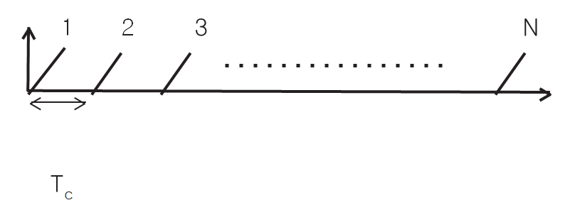
이 처리 기법의 예로 레이더와 동일한 거리에 있지만 v1 및 v2라는 다른 속도를 가진 두 물체가 아래에 설명되어 있다.
범위 FFT는 반사 처프 세트를 처리하여 동일한 위치에 있지만 각각 다른 위상을 가진 N개의 피크 세트를 생성하여 이러한 두 물체의 위상 기여도를 통합한다(이러한 각 물체의 개별 위상 기여도는 그림 8에 빨간색 페이저와 파란색 페이저로 표현되어 있다).
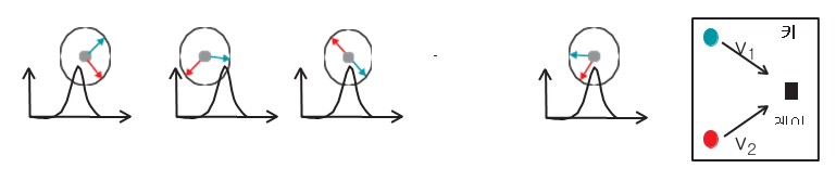
도플러 FFT라고 하는 두 번째 FFT는 표시된 것처럼 N 페이저에서 두 물체를 확인하기 위해 수행된다.
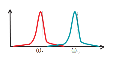
ω1 및 ω2는 해당 물체의 연속 처프 간 위상 차이에 해당한다(방정식 13).
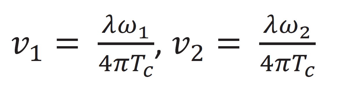 (13)
(13)속도 해상도
개별 푸리에 변환 이론에 따르면 Δω= ω 2 ? ω 1 >2π/N radians/sample일 경우 두 개의 개별 주파수 ω 1 및 ω 2를 확인할 수 있다.
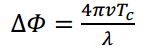 (방정식 10), 정확히 속도분해능(Vres)
프레임 기간이라면 단, Tf = NTc(방정식 14):
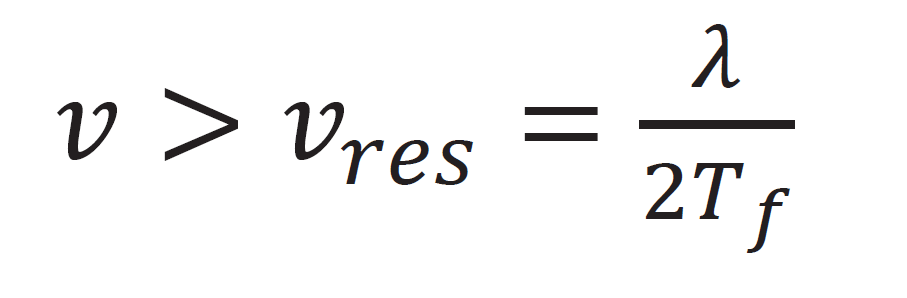 (14)
(14)레이더의 속도 분해능은 프레임 시간(Tf)과 반비례한다.
각도 감지
FMCW 레이더 시스템은 그림 10에 나와 있는 것처럼 수평면을 사용하여 반사 신호 각도를 추정할 수 있다. 이 각도를 도래각(AoA)이라고도 한다.
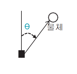
각도 추정은 물체 거리의 작은 변화가 범위 FFT 또는 도플러 FFT 피크의 위상 변화를 초래하는 관찰을 기준으로 한다. 이 결과는 그림 11에 표시된 것과 같은 두 개 이상의 RX 안테나를 사용하여 각도 추정을 수행하는 데 사용된다. 각 안테나와 물체의 미분 거리는 FFT 피크에서 위상 변화를 가져온다. 위상 변화를 사용하여 AoA를 추정할 수 있다.
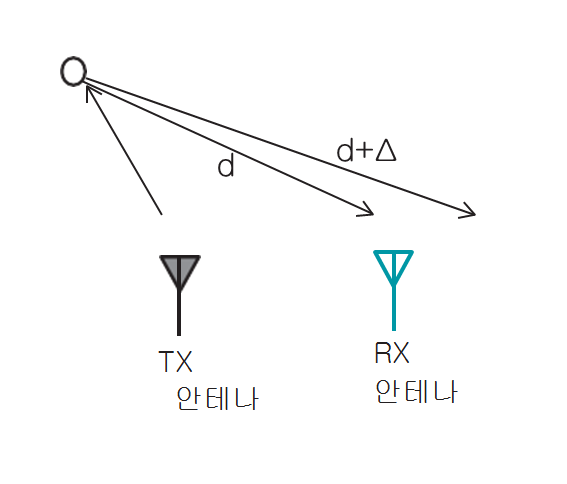
이 구성에서 위상 변화를 방정식 15와 같이 구한다.

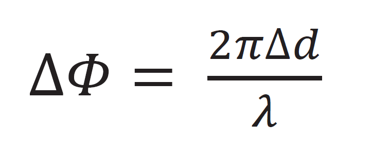 (15)
(15)평면 파면을 가정할 때 기본 지형은 Δd = lsin(θ)을 보여준다. 여기서 l는 안테나 사이의 거리다. 따라서 도래각(θ)은 방정식 16에서 측정된 ΔΦ로 계산할 수 있다.
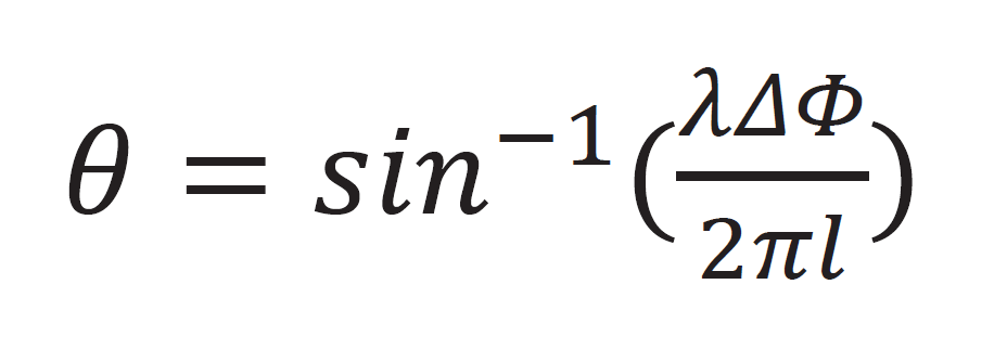 (16)
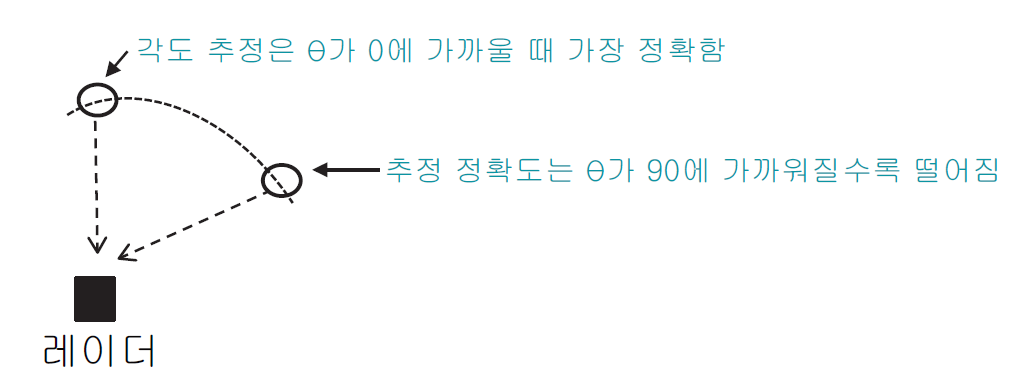
(16)ΔΦ는 sin(θ)에 종속된다는 점에 유의해야 한다. 이를 비선형 종속성이라고 한다. sin(θ)은 θ값이 작을 때만 선형 함수를 사용하여 근사치로 계산된다:
sin(θ) ~ θ.
따라서 추정 정확도는 그림 12에 나온 것처럼 AoA에 따라 달라지며, θ값이 작으면 더 정확하다.
최대 시야각
레이더의 최대 시야각은 레이더가 추정할 수 있는 최대 AoA로 정의된다. 그림 13을 참조할 수 있다.
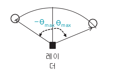
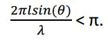 에 해당한다.
방정식 17은 l 간격의 두 안테나가 제공할 수 있는 최대 시야각이 다음과 같다는 것을 보여준다.
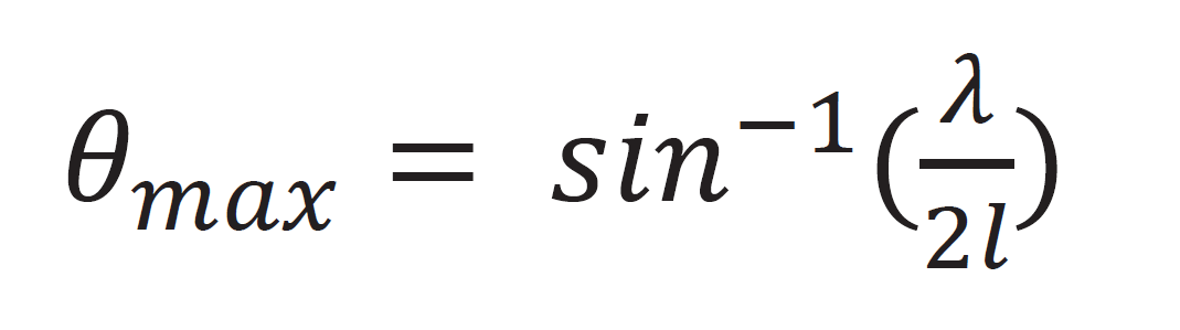 (17)
(17)두 안테나 사이의 간격 l = λ/2는 최대 시야각 ± 90°를 초래한다.
텍사스 인스트루먼트 mmWave 센서 솔루션
아시다시피 FMCW 센서는 RF, 아날로그 및 디지털 전자 부품을 함께 사용하여 근처에 있는 물체의 범위, 속도 및 각도를 파악할 수 있다.
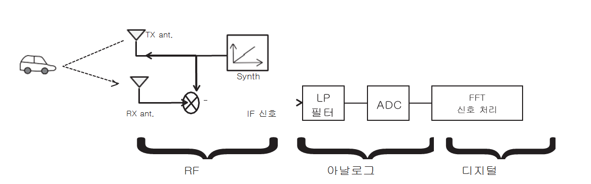
TI의 RFCMOS mmWave 센서는 mmWave RF 프론트 엔드 및 MCU/HWA/DSP 처리 백 엔드에 유연성과 프로그래밍 기능을 구현하여 기존의 SiGe 기반 솔루션과 차별화를 꾀했다. SiGe 기반 솔루션은 제한된 수의 처프만 저장할 수 있고, 실제 프레임 중에 처프와 처프 프로필을 업데이트하려면 실시간 개입이 필요한 반면, TI의 mmWave 센서 솔루션은 프레임이 시작되기 전에 4개의 프로필을 사용하여 512개 처프를 저장할 수 있다. 이러한 기능 덕분에 TI의 mmWave 센서를 여러 구성으로 쉽게 구성하여 현장에서 유용한 데이터를 최대한 많이 추출할 수 있다. 개별 처프와 처리 백 엔드는 범위 확대, 속도 증가, 분해능 개선 또는 특정 처리 알고리듬과 같은 실시간 애플리케이션 요구 사항에 맞게 “즉석에서” 맞춤 구성할 수 있다.
TI mmWave 센서 포트폴리오는 고성능 프론트 엔드 레이더 AWR1243 센서부터 단일 칩 레이더 AWR1443 센서 및 AWR1642 센서까지 다양하게 구성된다. 설계자는 AWR mmWave 포트폴리오 제품으로 ASIL(Automotive Safety Integrity Level) B를 구현하는 ISO 26262를 비롯한 ADAS (첨단 운전자 보조 시스템) 및 자율 주행 안전 규정을 충족할 수 있다.
산업용 TI mmWave 센서 포트폴리오는 두 가지 단일 칩 장치로 구성된다. IWR1443 mmWave 센서는 레이더 신호 처리를 위한 하드웨어 액셀러레이터를 포함하고 있으며, IWR1642 mmWave 센서는 DSP를 사용하여 필요한 처리를 수행한다. DSP는 더 뛰어난 유연성을 제공하며, 추적 및 분류와 같은 다른 더 높은 수준의 알고리듬을 소프트웨어에 통합할 수 있게 지원한다. 이러한 단일 칩 디바이스는 물체의 범위, 속도 및 각도 등에 관한 매우 정확한 데이터에 간편한 액세스를 지원하여 스마트 인프라, 공장 및 건물 자동화 제품의 Industry 4.0, 자율 주행 드론 등 성능과 효율성이 요구되는 유망 애플리케이션에서 고급 감지를 지원한다.
텍사스 인스트루먼트는 다음을 포함한 산업용 및 오토모티브용 mmWave 센서 제품을 제작하는 엔지니어를 위한 완전한 개발 환경을 제공한다.
mmWave 제품, 툴 및 소프트웨어에 대해 자세히 알아보려면 www.ti.com/mmwave를 방문하면 된다.

Comments
Related news

ADI Simplifies RF, Microwave, and Millimeter-Wave Design and Evaluation Processes
Analog Devices (hereinafter ADI) announced that it is collaborating with X-Microwave LLC, a specialist in RF and microwave modular building blocks, to enable RF developers to efficiently and rapidly evaluate RF components and prototype signal chains. As the first phase of the collaboration between the two companies, X-Microwave will provide over 250 ADI RF, microwave, and millimeter-wave products as drop-in modular building blocks. ADI maintains a portfolio consisting of over 1,000 types of RF, microwave, and millimeter-wave components. It also provides software and support tools that RF engineers need to develop complete signal chain solutions spanning from DC to 100 GHz tailored to their respective applications. Additionally, signal chains can be constructed simply by arranging modular configuration blocks and simulating the designed system using X-Microwave's online tools. This approach stands in sharp contrast to the conventional cumbersome system development method that requires connecting multiple evaluation boards using dozens of cables. This enables designers to streamline the design process while reducing time-to-market and development costs.
2017.06.15by 김자영 기자
[Contribution] How to design a flexible ADAS radar sensor
TI's AWR1x millimeter wave (mmWave) sensor portfolio enables developers to drive more safely and conveniently. Based on a mmWave sensing architecture (Figure 2), the AWR1x sensor integrates radio frequency (RF) and analog functions along with digital control functions into a single chip.
2017.07.20by 명세환 기자
[Contribution] Understanding the Difficult Millimeter-Wave System Design (Part 1)
A complete mmWave radar system includes transmission (TX) and reception (RX) radio frequency (RF) components, analog components such as clocking, digital components such as ADC (analog-to-digital converter), MCU (microcontroller), and DSP (digital signal processor). Traditionally, these systems were implemented with discrete components, which increased power consumption and overall system cost. Due to complexity and high frequency, system design was also challenging. Texas Instruments (TI) addressed these challenges and designed CMOS (complementary metal-oxide-semiconductor) based mmWave radar devices that integrate TX-RF and RX-RF analog components such as clocking and digital components such as ADC, MCU, and hardware accelerators. Some product families in the TI mmWave sensor portfolio have integrated DSP for additional signal processing capabilities.
2017.08.18by 명세환 기자
[e4ds Tech Day 2026 ⑨] Sim Sang-gyu, Autocrypt CTO: "In the Physical AI Era, Automotive Security Must Extend Beyond the Vehicle"
At e4ds Tech Day 2026, Sim Sang-gyu, CTO of Autocrypt, explained automotive cybersecurity strategies in the era of Physical AI and SDV (Software-Defined Vehicle). Automobiles are evolving as part of an ecosystem connected to AI, cloud, chargers, IoT, and robots, and he emphasized that the scope of security must expand beyond the vehicle interior to the entire connected environment. In particular, AI model tampering, adversarial attacks, OTA updates, and EV charger hacking were identified as major threats. He explained that response measures require zero trust, AI model integrity protection, intrusion detection, Security by Design and Default, and full lifecycle security management, and that proactive security system establishment beyond regulatory compliance is critical for securing future mobility competitiveness.
2026.10.12by 배종인 기자

Practical HIL Construction Strategy for Automotive and Off-Highway Controller Validation
As vehicle E/E architecture transitions to zonal structures and shifts to software-defined vehicles (SDV), the number of controllers (ECUs) requiring validation and software complexity are surging dramatically. Meanwhile, real vehicle testing cannot provide repeated verification under identical conditions and entails lead time and safety concerns. This white paper explains the principles of HIL (Hardware-in-the-Loop) validation and the structure of the NI platform composed of PXI, SLSC, and VeriStand, and through two actual implementation cases—Camera Record & Replay HIL for In-Cabin Monitoring Controller (ICMU) and Forklift Controller (VCU) HILS—describes how controller-level regression testing becomes possible. Additionally, it explicitly states application boundaries and limitations, such as lack of A2B support.
2026.10.12by 편집부